Schrodinger’s Wave Model
of the Atom – A Physical Interpretation.
Doug Marett, 2022
A .pdf version is available here
It has
often been argued that one of the most problematic aspects of Quantum Mechanics
has been the inability to describe its tenets in a realistic way – realism and physicality
have been replaced by statistical and mathematical representations which
divorce the initiate from rational understanding. One could argue that the theory
of wave-particle duality of Quantum Mechanics is one of the most problematic in
this regard, as conceptually it leads to paradoxes and contradictions if one
attempts to understand it at face value. One is left instead with hand-waving
and comforting words suggesting that the incomprehensibility of it all is
perfectly normal – the “6 impossible things before breakfast.”
However, this is not necessarily how it
was originally intended. In Schrodinger’s Wave Mechanics that led to the most
accurate description of the atom to date, his intention was to portray the atom
with “ Anschaulichkeit “ (picturability)1. We will argue herein that the
wave-particle dualism that emerged from the Copenhagen interpretation of
Quantum Mechanics was an incongruous revision of Schrodinger’s original
“realism”. For this reason we would like to revisit Schrodinger’s spherical
wave model and explain it in a picturable way, while also addressing some of
the issues brought forward by his detractors.
In 1925-1926
Schrodinger, inspired by the work of Louis de Broglie, sought to find a way to
describe the electron orbitals using a new model he referred to as Wave
Mechanics2. In de Broglie’s theory the electron
waves were considered to follow the orbit of the electron around the nucleus
and an integral number of wavelengths would need to fit the circumference of
each orbit. Schrodinger attempted instead to imagine electromagnetic (EM) waves
circulating around the nucleus spherically, a process which is hard to imagine
using ray optics, but is possible using wave-fronts. Schrodinger elucidated
this physical model in his Nobel Prize lecture in 1933 entitled “The
fundamental idea of wave mechanics.”3 The lecture is remarkable in that
although he won the prize for a quantum mechanical description of the atom, the
lecture is almost entirely about optics! The fundamental idea that led
Schrodinger to his discovery can be described best in a quote from his lecture
below:
“Instead of the electrons we introduce hypothetical waves,
whose wavelengths are left entirely open, because we know nothing about them
yet. This leaves a letter, say a, indicating a still unknown figure, in our
calculation. We are, however, used to this in such calculations and it does not
prevent us from calculating that the nucleus of the atom must produce a kind of
diffraction phenomenon in these waves, similarly as a minute dust particle does
in light waves. Analogously, it follows that there is a close relationship
between the extent of the area of interference with which the nucleus surrounds
itself and the wavelength, and that the two are of the same order of magnitude.
What this is, we have had to leave open; but the most important step now
follows: we identify the area of interference, the diffraction halo, with the
atom; we assert that the atom in reality is merely the diffraction phenomenon
of an electron wave captured as it were by the nucleus of the atom. It
is no longer a matter of chance that the size of the atom and the wavelength
are of the same order of magnitude: it is a matter of course.” 3 p. 314
So in
Schrodinger’s conception the electron is quite literally the EM wave
diffraction halo surrounding the nucleus. We will try to picture what this
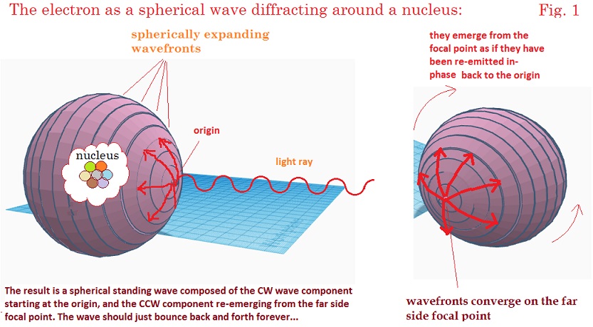
would look like with
some diagrams below. In this image an EM wave approaches a nucleus,
and following Huygens principle, forms an expanding
wave-front beginning at the origin which curves around the spherical path of
the diffraction halo. On the opposite side of the halo, it converges again to a
point, where the wave-fronts pass through each other and begin to travel back
again along the same spherical trajectory in reverse. The result is a spherical
standing wave that oscillates indefinitely. This conception solves at least a
first point regarding how an electromagnetic wave could form a continuous
spherical shell. The process constraining the EM wave-fronts to follow the
curved path might seem implausible when considered in terms of geometric
optics, but Schrodinger felt that this form of optical science might not be the
best to describe diffraction around microscopic objects where the wavelength
was on the order of the dimensions of the object. Schrodinger saw that there
was a close analogy between Hamilton’s principle and Fermat’s optical
principle, and that the former could be used to express the proposed undulatory
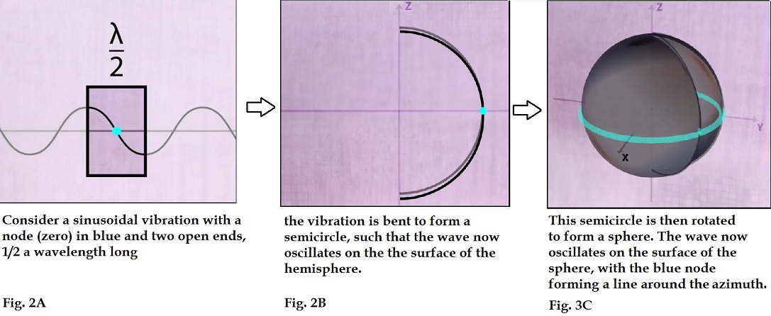
phenomenon in a manner better than via geometric optics alone. Consider an
undulatory vibration on a string as shown below in figure 2A.4 This will serve as our analogy of Schrodinger’s model of the electron EM
wave. The portion of the string highlighted in the box is ½ wavelength, which
has one node at the zero crossing (blue), and two open ends at positive and
negative. If this vibrating string is bend into a semicircle, it will then
appear as in fig 2b, oscillating up and down with respect to the node. If this
semicircle is then rotated around to form a sphere, then we have our spherical
oscillator with the upper and lower portions of the sphere oscillating between
positive and negative about the azimuthal nodal line at the equator of the
sphere.
As the distance around the circumference
from pole to pole is ½ wavelength, then the shell would form a standing wave
with at a snapshot in time the positive part of the waveform is at one pole and
the negative part at the other, as shown below mapped on a unit sphere:
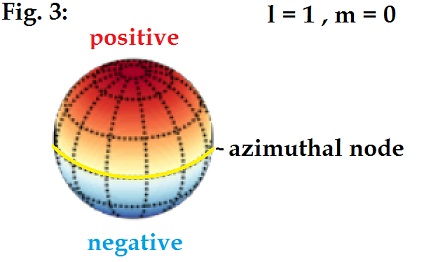
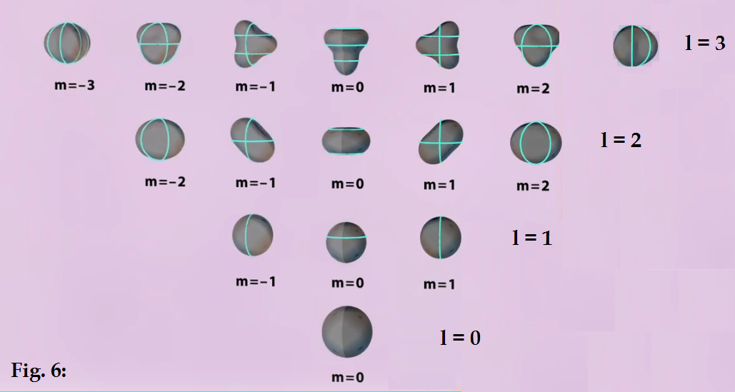
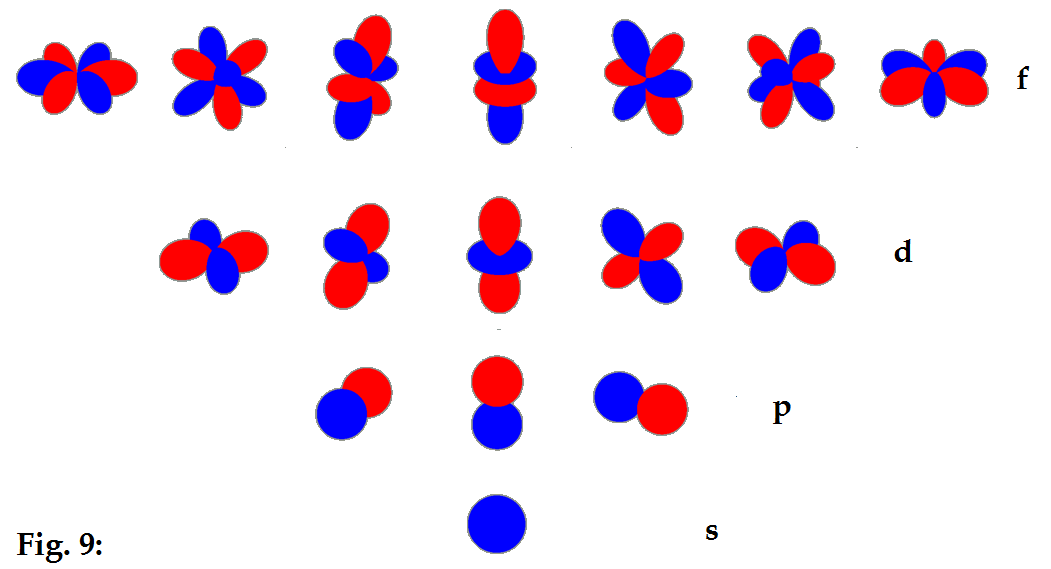
The spherical harmonics as described by Schrodinger follow a
series where the letter l designates the number of nodes on the sphere. The
first level, l=0, corresponds to the s orbital and has zero nodes, so the
oscillation comprises a ¼ wave from pole to pole. The second level l =1
corresponds to the p orbital with 1 node, so ½ wavelength from pole to pole.
The l =2 (d orbital, 2 nodes) is 1
wavelength from pole to pole, and finally the l =3 (f orbital, 3 nodes) is 1.5
wavelengths from pole to pole. This is shown diagrammatically below in Fig 4
starting with the wave vibration shown on a linear string with its nodes in
blue.
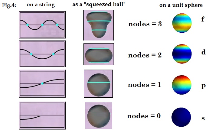
Then in the middle, the corresponding spherical wave is shown
as a ball squeezed by the wave. On the right, the wave polarization is shown
mapped onto the unit sphere, where the red contours show where the positive
charge is, the blue the negative the intensity of the colour reflecting the
intensity of the charge. The advantage of the unit sphere projection is that it
shows the “path” of the waves as following the surface of the sphere.
These harmonics can be expanded further if we consider that
the azimuthal nodes can also rotate about the z axis. This is shown below. The
l = 0, m =0 harmonic has
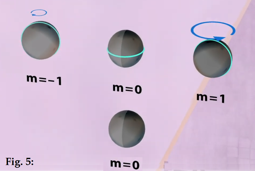
no node so it can’t be rotated, but the l =1 can have its
azimuthal nodal line rotated clockwise or counter-clockwise about the z-axis,
leading to three possible modes m= -1, 0, 1. The same is true of the higher
harmonics : l =2 having 2 nodal lines has three possible modes -2, -1, 0, 1, 2
where 0, 1, or 2 of the nodal lines are rotated clockwise or CCW about the z
axis. For l=3, there are 7 possible modes. These are all shown diagrammatically
below in Fig. 6. Again, in this representation, we are showing the spheres as
“squeezed balls” with the azimuthal nodal lines of the waves shown in blue.
When Fig. 6 is represented as spherical waves with their
polarization intensity projected on the unit sphere, similar to in Fig. 4, they
appear as below (Fig. 7):
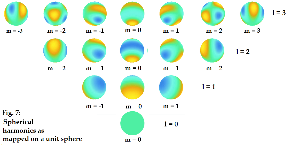
In this case yellow represents the most positive crest of the
waves, blue the most negative crests, again, the colour intensity maps the
charge intensity in a topological way.
It is important to point out the meaning of electron “spin”
in this model. The rotation of the azimuthal nodal line(s) around the z-axis corresponds
to extrinsic
spin. So for each azimuthal line that rotates, the spin increases by ½ or - ½
depending on the rotation direction. The
base oscillation of the wave on the sphere corresponds to intrinsic spin. So an
orbital with 2 rotating azimuthal lines would have a spin of either +1 ½ or – 1
½.
There is another
way of displaying spherical harmonics. They can be plotted as the magnitude of
the function along each direction to define a radial distance, and then plot
the function at that radial distance. If we were to regard the polarity of the
waves on the sphere as a distribution of electric field, then the radial
distance plot would show the field intensity in space around the sphere.
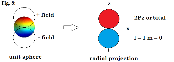
This radial projection is shown below for the orbitals from s
through f.
These are then the familiar shapes of the electron orbitals
expressed as solutions of Schrodinger’s equation for the electron.
In Schrodinger’s writings, he repeatedly emphasized that the
wave-function Y was describing
a physical electromagnetic wave, which is not what the current consensus view
of what the orbitals are in quantum mechanics. For example, in Schrodinger’s
“collected Papers on Wave Mechanics”, he stated:
“It is necessary to ascribe to Y a physical, namely an electromagnetic , meaning in
order to make the fact that a small mechanical system can emit electromagnetic
waves of a frequency equal to a term difference (difference of two proper
values divided by h) intelligible at all, and further, in order to obtain a
theoretical statement for the intensity and polarization of these
electromagnetic waves.” Ref 3, Abstract, P. x
And also:
“A definite
Y
distribution in configuration space is
interpreted as a continuous distribution of electricity (and of electric
current density) in actual space. If from this distribution of electricity we calculate the component of
the electric moment of the whole system in any direction in the usual way…” Ref 3, Abstract, P. x
It is important to note that Schrodinger rejected the notion
of the electron as a “point charge.” As shown above, his interpretation is that
the electron was the spherical harmonic, i.e. the “diffraction halo” around the
nucleus, not individual point charges located indeterminately in a statistical
probability distribution around the nucleus. On this matter, he said:
“We shall
be obliged to attempt to take over the idea of Uhlenbeck and Goudsmit into wave
mechanics. I believe that the latter is a very fertile soil for this idea,
since in it the electron is not considered as a point charge, but as
continuously flowing through space, and so the unpleasing conception of a “
rotating point-charge ” is avoided.” Ref. 3 P, 64.
And in his interpretation of the square of the wavefunction,
he stated explicitly that this refers to the density of electricity:
“According to the hypothesis of wave mechanics, which up to now has always proved trustworthy, it is not the Y-function itself but the square of its absolute value that is given a physical meaning, namely, density of electricity.” Ref. 3, P. 126
Addressing further shortcomings
of the model:
Having come this far, we recognize there are some further issues
that arise with taking Schrodinger’s model literally. These are:
1)
- How
do we account for unipolar charge when the waves are bipolar?
2)
- How
do we obey Pauli’s exclusion principle – 2 electrons per orbital?
3)
- How
do we explain pair production/annihilation?
4)
- What
about the magnetic fields?
Let’s consider the
spherical harmonic of figure 3. If it was genuinely an electromagnetic wave
whose wave-front advances around the sphere to form a standing wave, then the object
would be bipolar, not single-charged as expected for an electron or positron. Further,
it would fill the entire orbital rather than leaving space for another electron
– as we know from Pauli’s exclusion principle, each orbital can hold up to two
electrons. If each electron is a unit sphere, then this would require two unit
spheres to overlap per orbital to properly fill the electron placements. In an attempt to find a model that fits, we
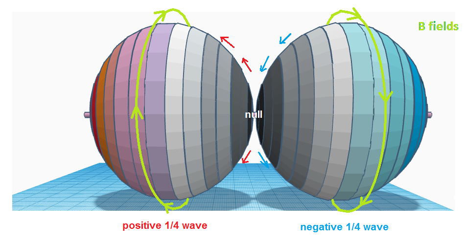
will examine an example of two hypothetical ¼ wavelength (pole to pole) spherical
resonators as shown below, with the colours showing the charge and the green
band showing the magnetic field direction.
Fig. 10:
A ½ wave traverses the spheres with ¼ wave across one sphere and
then continues to the second ¼ of the wave on the other. The wave starts at the
right origin at a negative peak, travels to the null point at the opposite
pole, and then continues onto the left side resonator as the positive-going
side of the wave, reaching a positive peak at the leftmost pole. The magnetic
field for each sphere is shown – the magnetic fields counter-rotate with
respect to each other obeying the right hand rule. Now imagine that this ½ wave
traverses only the right side sphere as a forward/ reverse standing wave– it
would go from the rightmost pole to the null at the center, then pass through
the focal point and head back towards the right side pole, but this time as the
positive going side of the wave. This would be equivalent to taking the left
side sphere shown above, rotating it 180 degrees, and superimposing it on the
right side sphere. The fields on the right side sphere would then comprise two
¼ wave sections of the same wave that are opposite in polarity and overlapping,
and their magnetic fields would now be co-rotating.
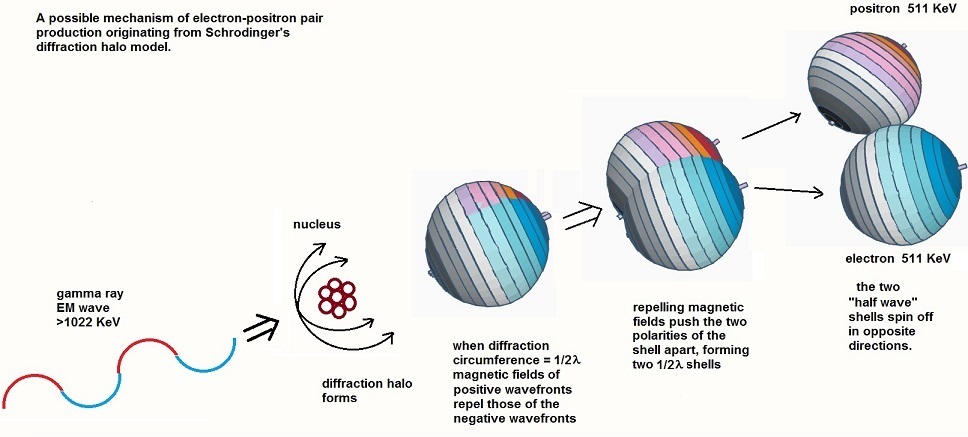
We could argue that this latter scenario would be forbidden, since in vortex theory co-rotating magnetic vortices repel, so the positive going ¼ wavelength would be pushed away from the negative going ¼ wavelength that it overlaps. I speculate that it is this kind of process that could potentially lead to electron-positron pair production if the correct conditions, currently not fully understood, could be met. The electromagnetic wave, on being constrained in a diffraction halo, and then forced to overlap on itself such that its magnetic fields are set up in a repulsive conformation, would literally break the EM wave into two “half-wave” components, one positive and one negative, almost like a form of electronic rectification. In this scenario, each shell oscillates between positive and null, or negative and null, but not positive and negative. This is not a process of reflection at the focal point of each sphere – rather, the wavefront passes through the focal point and continues in the opposite direction on the sphere unabated, but the wave only oscillates between negative and zero around the new electron sphere (or positive and null for the positron), so the new azimuthal node becomes the potential half way between these two. So the oscillation remains a sine wave on both spheres, but their reference to the original “zero” level is changed. Their forced separation into two entities is then conceived of as being something like that shown diagrammatically in the figure below.
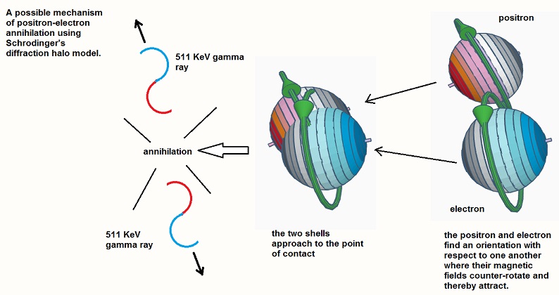
Conversely, if the two shells, positive and negative, then re-approach one another in the attractive orientation where the magnetic fields are counter-rotating (as shown in the next figure) they will be pulled together and will annihilate, recreating the original EM waves which will be emitted from the annihilation site.
Again we can speculate on the process of annihilation,
knowing that it would require that energy is conserved. The transformation from
one state (the shells) to the new state (the linear gamma rays) might best be
explained using the Maxwell-Lorentz theory referred to by Schrodinger in his
writings.2
This theory would define the electric field as a strain in the medium between
the magnetic fields7, and thus the environment becomes
part of the annihilation sequence. The complete cancellation of the magnetic
field loops would then lead to a release of the strain energy into the surrounding
medium, where new oscillating magnetic fields would be reconstituted to allow
the energy to propagate away as high frequency gamma rays.
With this speculative
model of the unipolar wave spherical
shell resonator, we note a few things. With the shells shown in Fig 11 and 12,
when the origin is a peak, then the opposite pole is a null. This ½ wave
circumference shell might best match the 2p orbital. We first contrast this
with a shell where the circumference is equal to one full bipolar EM wavelength, so the left pole is positive and the right
pole is negative, as was originally pictured by Schrodinger in for example fig.
3. When expressed this way, the radial electric field intensity from each
positive and negative segment of the shell adds up to form in radial projection
two lobes, one positive and one negative, similar to the shape of one segment
of the 2p orbital, as shown below.
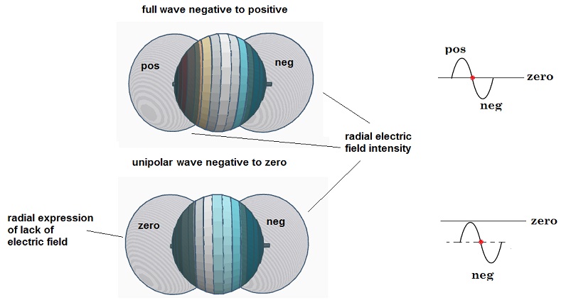
However, if the same exercise is performed on the unipolar
wave shell, the same kind of lobes can be used to express the charge, where the
negative lobe expresses the electric field as “furthest from zero negative” and
the zero lobe expresses “closest to zero in the positive direction”. The
spherical shell in this unipolar form can then at least meet the necessary
condition that the charge is always positive or always negative, but never
both.
The advantage of this latter shell is that
the zero lobe is essentially empty, so it can be filled by another electron standing
wave in the opposite orientation, matching the quantum criteria that two
electrons can be in the same 2px, 2py, or 2pz orbital but not in the same
position. This would effectively be two unipolar
wave vibrations in anti-phase on the same unit sphere. The magnetic fields of
the two vibrations would always be counter-rotating, thus attractive and
cancelling, whereas the charges would be repulsive, forming a balance of
forces.
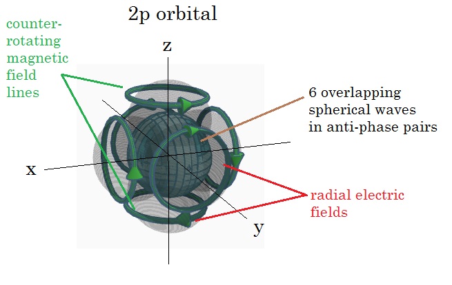
When all 6 are
added in the x,y,and z orientations, the electric field density would look
somewhat like below, corresponding to the 2px, 2py and 2pz orbitals, as shown
distributed on the spherical harmonic unit sphere. Each pair of electron
standing waves would be 180 degrees out of phase on the unit sphere, forming 6
magnetic fields which counter-rotate for each pair and thus cancel out. The
resulting electric charge distribution is then cloudlike and symmetrically
distributed about the sphere.
Similar rules apply to the other orbitals as are summarized
below:
s = ¼ lambda from pole to pole unipolar wave on the unit
sphere
d = ½ lambda from pole to pole unipolar wave on the unit
sphere
d = 1 lambda from pole to pole unipolar wave on the unit
sphere
f = 1.5 lambda from pole to pole unipolar wave on the unit
sphere
The model solves some issues in an obvious
way – electrons do not travel in orbits, but instead EM waves simply pass over
each other on spherical shells. This eliminates the issue of collision since
the EM waves can pass through each other without resistance. Pauli’s exclusion
principle is met since electron shells overlap in a manner such that
counter-rotating magnetic fields cancel, thus balancing charge with magnetic
attraction. The electrons don’t radiate energy in part since they don’t move in
a conventional sense. However the wavelengths do not appear to define a
standard physical size of the orbitals – the s or p orbital radius differs from
atom to atom, and is also much larger in dimensions than the wavelength of the
511 KeV gamma ray that created it. So in order to take the model literally, we
must imagine that each orbital would have to follow the rules of pole to pole
wavelength as set above, but the value of this wavelength is a variable that
depends on the specific conditions of the nucleus the electron shell surrounds.
We have herein
attempted to visualize a possible model of the Schrodinger electron orbitals
that is true to Schrodinger’s original vision, at least for the figures 1-9. In
our “Addressing further shortcomings of the model” we have speculated on some
possible revisions that could potentially make the model compatible with
Pauli’s exclusion principle, pair production /annihilation, and proper charge
expression. As a final point, we would also like to note that Schrodinger’s
spherical wave hypothesis can also be applied to the nucleus. This is because the nucleus has been
discovered to have a shell structure similar to that of the electrons, with the
protons and neutrons existing in s, p, d, f, g orbitals as was first proposed
by Maria Goeppert Mayer, who received the Nobel prize in Physics for this work
in 1963 along with Hans Jensen. This then allows for all of the stable atomic
particles to potentially be composed of spherical standing wave shells, and, to
follow that to its logical conclusion, probably all stable particles with mass.
Schrodinger’s model opens the door to the notion that the “particle” doesn’t
exist at all in the conventional sense, that the underlying substratum of the
universe is the medium in which these waves move, rather than the universe
being entirely particulate. This discussion can by no means answer all of the
questions and issues that arise from his model, but that hasn’t been our
purpose, rather I have attempted here to put Schrodinger’s model into a rough form
that can be comprehended visually, to be true to his notion of “ Anschaulichkeit. “
References:
1) Bitbol, Michel, “Schrodinger’s Philosophy of Quantum
Mechanics”, Boston
Studies in the Philosophy of Science Volume 188, Kluwer Academic Publishing,
1996, P. 1-37.
2) Schrodinger, Erwin, “Collected papers on Wave Mechanics”, Blackie &Son, Glasgow, 1928.
3) Schrodinger, Erwin,” The fundamental idea of wave
mechanics”, Nobel
Lecture, Dec. 12, 1933.
4) Spherical Harmonics (U2-05-05)
tutorial video. QuantumVisions (WWU Münster)
5) Reference 1, (ref) P.12
6) Reference 1, (ref) P.13-14.
7) Maxwell, James Clerk, “On Physical Lines of Force”. Philosophical Magazine, Vol XXI,
p. 451-516. 1865.
8) Maria Goeppert Mayer Biographical, nobelprize.org